Welcome to another deep dive into algorithmic problem solving! Today, we are tackling a classic problem from the world of finance: the Best Time to Buy and Sell Stock with Cooldown. This article will walk you through understanding the problem, exploring an efficient solution using dynamic programming, and offering a challenge for those eager to test their skills further.

If you’re just joining us, it might be helpful to catch up on the previous entries. Want to see more problem-solving techniques? Follow me here on my blog!


Understanding the Problem
You are given an array prices where prices[i] is the price of a given stock on the ith day. The goal is to find the maximum profit you can achieve by completing as many transactions as you like (i.e., buying and selling one share of the stock multiple times) with the following restriction:
After you sell your stock, you cannot buy stock on the next day (i.e., you must observe a cooldown period of one day).
Example 1:
Input: prices = [1,2,3,0,2]
Output: 3
Explanation: transactions = [buy, sell, cooldown, buy, sell]
Example 2:
Input: prices = [1]
Output: 0
With the problem defined, let’s delve into efficient solutions to maximize our profit.
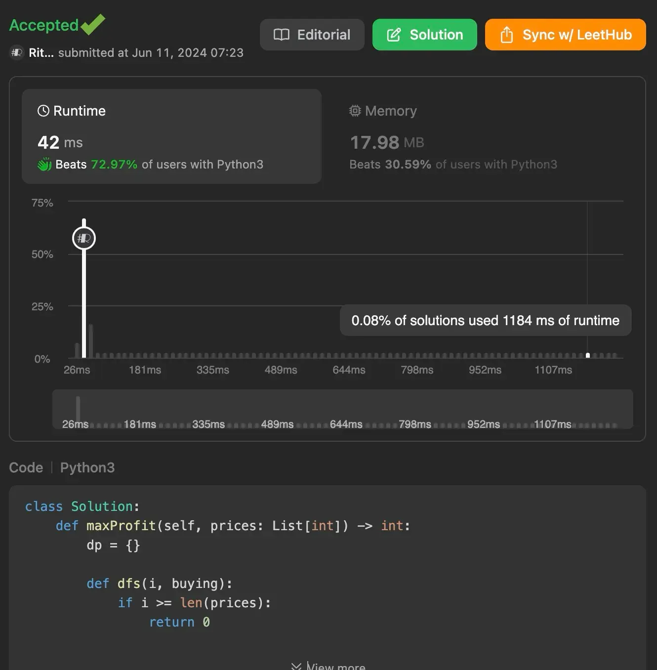
Using Efficient Approach 1: Depth-First Search with Memoization
The first efficient approach leverages Depth-First Search (DFS) combined with memoization to explore all possible states and transitions in our trading strategy. This ensures that we don’t recompute results for the same state, thus optimizing our solution.
def maxProfit(self, prices: List[int]) -> int:
    dp = {}

    def dfs(i, buying):
        if i >= len(prices):
            return 0

        if (i, buying) in dp:
            return dp[(i, buying)]

        cooldown = dfs(i + 1, buying)
        if buying:
            buy = dfs(i + 1, not buying) - prices[i]
            dp[(i, buying)] = max(buy, cooldown)
        else:
            sell = dfs(i + 2, not buying) + prices[i]
            dp[(i, buying)] = max(sell, cooldown)

        return dp[(i, buying)]

    return dfs(0, True)
Explanation
- We use a dictionary
dpto store the results of subproblems. - The dfs function recursively computes the maximum profit starting from day
iwith the state of either buying or selling. - If
iexceeds the length ofprices, it returns0, indicating no more profit can be made. - For each state, we calculate the profit of either buying or selling based on the current state and the next possible states.
- Since we can buy immediately and have to wait a day after selling, we increament the
iby2when selling. - Memoization is used to avoid recomputation, storing results of each state
(i, buying)indp.
Time Complexity: O(n), where n is the number of days. Each state is computed once.
Space Complexity: O(n), for the memoization dictionary.
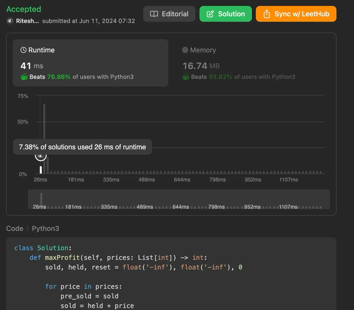
Using Efficient Approach 2: State Machine Approach
The second approach uses a state machine to track three states: sold, held, and reset. This method iteratively updates these states as we traverse through the prices, ensuring optimal profit calculation with linear complexity.
def maxProfit(self, prices: List[int]) -> int:
    sold, held, reset = float('-inf'), float('-inf'), 0

    for price in prices:
        pre_sold = sold
        sold = held + price
        held = max(held, reset - price)
        reset = max(reset, pre_sold)
    return max(sold, reset)
Explanation
- We initialize three states:
sold(maximum profit after selling a stock),held(maximum profit while holding a stock), andreset(maximum profit on a cooldown day). - For each
priceinprices, we update these states:soldis updated to the profit after selling the stock held the previous day.heldis updated to the maximum profit between holding the stock or buying new stock.resetis updated to the maximum profit between staying in cooldown or coming from a sold state.`
- Finally, we return the maximum of
soldandreset, as holding a stock at the end does not yield profit.
Time Complexity: O(n), where n is the number of days. Each state is updated once per day.
Space Complexity: O(1), as we use only a fixed number of variables.
Conclusion
In this article, we explored two efficient solutions to maximize profits in stock trading with a cooldown period. Both the DFS with memoization and the state machine approaches provide optimal solutions with linear time complexity. As you further hone your algorithmic skills, consider tackling variations of this problem to deepen your understanding and proficiency.
Understanding these methods enhances your problem-solving skills and prepares you for tackling similar challenges in coding interviews and competitions.
Found this helpful? Follow me for more leetcode adventures! Questions? React out via email.